Tungurahua Volcano Modeling & Simulation
Published:
In the fall of 2025, I was living in Seattle, working as a software engineer at SpaceX, and looking for a way to join my girlfriend in Palo Alto. I sent a number of emails to friends, coworkers, and past professors to inquire if they had leads on work that would allow me to work with both physics and software near Palo Alto.
One of those emails was to Prof. Eric Dunham, and lo and behold he responded:
I might have funding for a short term programmer position on a project related to explosive volcanic eruption modeling. I’ll need to check with my research admin when I’m back in the office next week about the project budget and to figure out exactly how I would be able to hire you.
We worked out the details, and after my last day at SpaceX in December of 2024 I began work with Prof. Dunham in January of 2025. In this writeup, I’ll describe some of the projects I worked on while working with Prof. Dunham and his PhD student Mario.
0.0 Intro
Prof. Dunham’s PhD student, Mario, was working to accurately model eruptions of Tungurahua, an active stratovolcano in Ecuador. Mario was working with a modified version of Quail, an open-source PDE solver that one of Prof. Dunham’s previous PhD students, Fred, had already modified to support modeling flow in a quasi-1D volcano conduit.
1.0 Slip weakening for plug
Background
We were working to model Vulcanian eruptions. Vulcanian eruptions are typically characterized by a solid plug forming in the conduit of the volcano, pressure building up beneath that plug, and ultimately a short, violent eruption after which a new plug forms in the conduit.
The project I was hired for was to implement a slip-weakening friction law for the volcano plug to the 1D conduit model. Prior to my arrival, the workflow for simulating an eruption was:
- Solve the steady state ODEs to arrive at the steady state initial conditions for the eruption.
- Apply those initial conditions to a dynamic model where the plug was effectively removed numerically causing the volcano to erupt.
My goal was to integrate the plug expulsion into the numerical model.
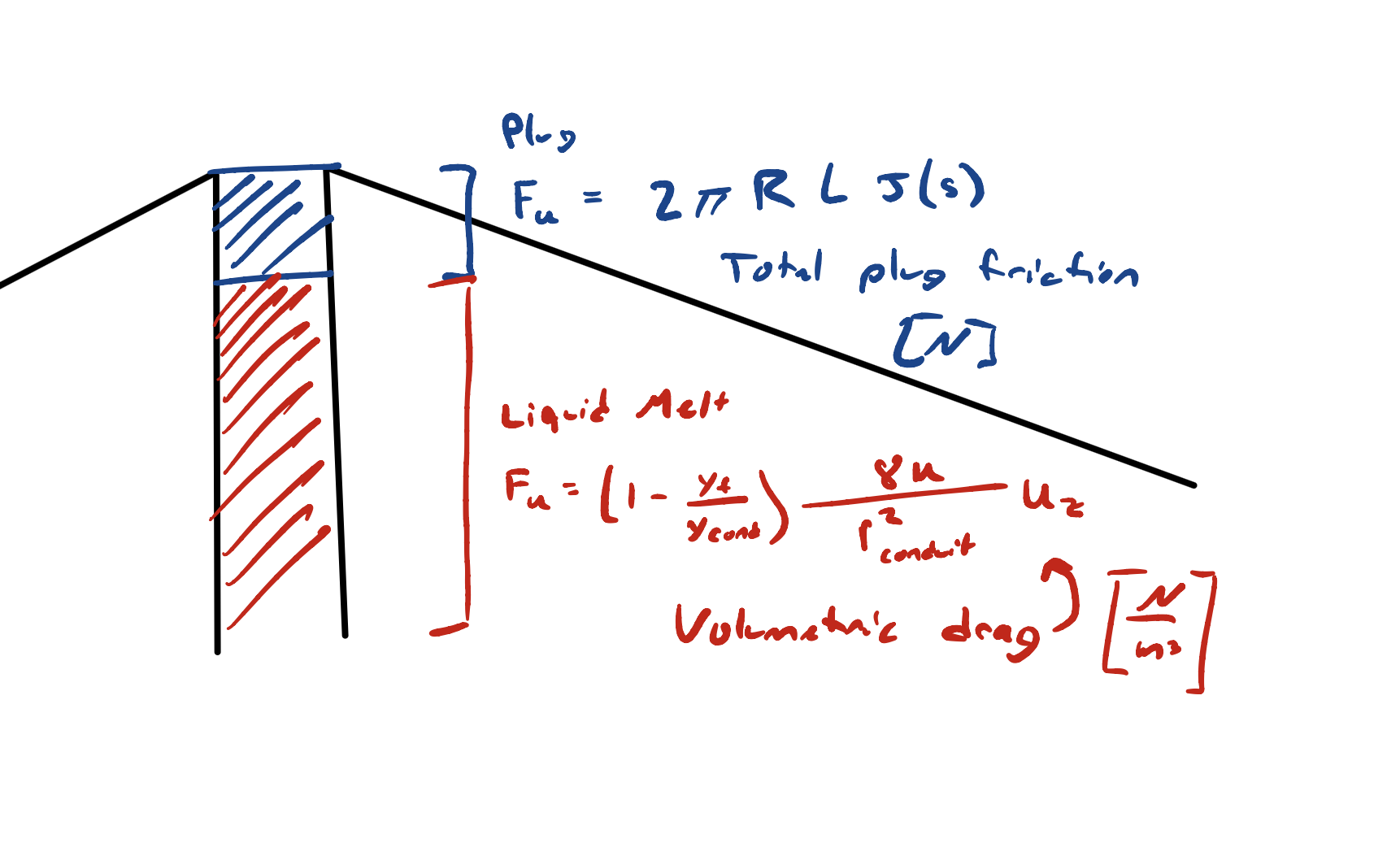
Specifically, I would add a feature to the quail simulation library to apply different friction laws to the solid plug and the liquid melt. For the plug, we apply a slip friction law that is the area where the plug contacts the conduit $\pi R L$ multiplied by $\tau(s(t))$, the wall shear stress where $s(t)$ is ‘slip’ or displacement as a function of time.
Prof. Dunham had previously applied “slip-weakening” with success to earthquake models and thought the mechanism would also be applicable to the volcano plug.
Implementation
To implement distinct friction laws for the plug and the melt, it is necessary to know the slip value for a specific position $x$ at a specific time $t$. Tracking slip as a function of position and time allows us to distinguish between the plug and the melt, and also provides an input for the slip weakening friction law.
The quail code models the quasi-1D conduit by conserving eight state variables:
- $y_a \rho$ - partial density air phase
- $y_{wf} \rho$ - partial density exsolved water
- $y_{cond} \rho$ - partial density condensed phase
- $\rho u_z$ - momentum
- $E$ - energy
- $y_{wt} \rho$ - partial density water, total
- $y_{crys} \rho$ - partial density crystals
- $y_f \rho$ - Fragmented condensed phase
Each of these variables is conserved according to various conservation equations. For example, the partial air density is conserved according to the equation:
\[\frac{\partial}{\partial t} (y_a \rho) + \frac{\partial}{\partial z}(y_a \rho u_z) = 0\]The conservation equation for our new slip variable is:
\[\frac{\partial}{\partial t} \rho s + \frac{\partial}{\partial z} s \rho u = \rho u\]I matched the implementation of other conserved state variables to add this new variable in this PR. With the new variable added, the next step was to implement the slip friction law. I added two variants: both the exponential law above and a linear slip weakening model.
\[\begin{align} \tau(s) &= \begin{cases} \tau_p - (\tau_p - \tau_r)(\frac{s}{D_c}) & s < D_c \\ \tau_r & s \geq D_c \\ \end{cases} \\ \tau(s) &= \tau_r + (\tau_p - \tau_r) \exp{-\frac{s}{D_c}} \end{align}\]Where $\tau_p$ and $\tau_r$ are parameters selected based on observational data from past eruptions. Then, I modified the slip friction source term to only apply friction in the “plug” region which could be deduced from our new ‘slip’ state variable. Similarly, I updated the viscous drag source term to only apply in the “melt” region.
Validation
To show that the slip-weakening force is working as expected, let’s consider a simplified model where the only forces at play are pressure, gravity, slip-weakening friction, and viscous drag. The resulting ODE for the slip of the plug:
\[\begin{align} M \ddot{s} &= A (p_0 + \Delta p(s)) - p_{atm}A - Mg - 2 \pi R L_p \tau(s) - \frac{8 \mu}{R^2} \dot{s} \\ \end{align}\]where $p_0$ is the pressure just below the plug and $\mu$ is viscosity. Solving for the steady state–where acceleration ($\ddot{s}$) and velocity ($\dot{s}$) are zero–we get:
\[\begin{align} 0 &= A p_0 - p_{atm}A - M g - 2 \pi R L_p \tau_p \\ p_0 &= p_{atm} + \rho g L_p + \frac{2 L_p \tau_p}{R} \end{align}\]With the specific values from our test problem we get:
\[\begin{align} p_0 &= 1e5 + \frac{2* 50 [m] * 1e6 [Pa]}{10 [m]} + 2.6e3 [kg/m^3] * 50[m] * 9.8[m/s^2] \\ p_0 &= 11.4e6 \\ \end{align}\]Further, if we wanted to calculate the expected pressure in steady state at the very bottom of the domain, we could do that with
\[\begin{align} p_L &= p_0 + \rho g * L_{c} \\ P_L &= 11.4e6 + 2.6e3 [kg/m^3] * 950 [m] * 9.8 [m/s^2] \\ P_L &= 36.6 [Pa] \end{align}\]When we run the numerical model with those steady state values as our initial conditions, we see that no slip occurs and the numerical steady state lines up very closely with the analytical results. That suggests that we have correctly implemented the zero velocity case.
Stability analysis
In the above example we appear to have a stable equilibrium. One question is: for what value of $D_c$ is the system unstable? That is to say, for what value of $D_c$ is:
\[\frac{|\frac{d F_f}{d s}|}{|\frac{d F_p}{d s}|} < 1\]Where $F_f$ is the force due friction between the plug and conduit walls and $F_p$ is force due to pressure of the liquid melt. When the condition above is met, that means that the force due to friction decreases more rapidly than the force due to drag decreases. As a result, we would expect that once the system starts slipping it will at least slip until $s = D_c$. The two forces can be expressed as:
\[\begin{align} F_f(s) &= 2 \pi R\tau(s) \\ F_p(s) &= A(p_0 - \Delta p(s)) \\ \end{align}\]For our analysis, lets assume a linear slip weakening law and assume that the compressible melt acts according to the law:
\[K = - L \frac{dP}{dL}\]Where K is the bulk modulus. We are able to write out the derivatives
\[\begin{align} \frac{d F_P}{ds} &= A * \frac{dP}{ds} = \frac{-A * K}{L_{c}}\\ \frac{d F_f}{ds} &= 2 \pi R L_p \frac{\tau_p - \tau_r}{D_c} \end{align}\]The instability condition above is met specifically when
\[\begin{align} D_c < \frac{L_{c} 2 \pi R L_p (\tau_p - \tau_r)}{A K } \\ D_c < \frac{2 L_{c} L_p (\tau_p - \tau_r)}{R K } \\ \end{align}\]Plugging in the problems specific to my toy problem I get:
\[\begin{align} D_c &< \frac{950 [m] * 50 [m] * 1e6 [Pa]}{10 [m] * 1e9 [Pa]} \\ D_c &< 4.7 \\ \end{align}\]In order to test, this result, I leave the initial conditions the same as the previous problem but I reduce $D_c$ to $3 [m]$. Sure enough that is sufficient to cause a small “eruption”
2.0 Lumped parameter model
For further verification and understanding, we decided it might be helpful to compare the results generated by Quail to the numerical solution of the ODE:
\[\begin{align} M_{eff} \ddot{s} &= A (p_0 + \Delta p(s) - p_{atm}) - 2 \pi R L_p \tau(s) - M_{eff} g - 4 \mu L_{c} \dot{s} \\ \ddot{s} &= \frac{A}{M_{eff}}(p_0 - p_{atm} - \frac{Ks}{L_{c}}) - \frac{2 \pi R L_p \tau(s)}{M_{eff}} - g - \frac{4 L_{c} \mu \dot{s}}{M_{eff}} \end{align}\]To calculate the viscous drag term, we assume the velocity in the melt increases linearly from zero at the bottom of the conduit to $u_z$ at the top. See my weekly notes from March where I discuss this.
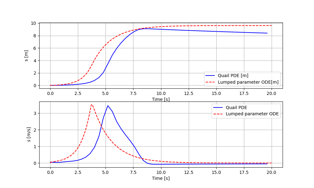 Lumped parameter model compared to Quail for the “slip” eruption simulated in section 1.
In addition to verification, we hoped the lumped parameter model would allow us to quickly test out a variety of values of: $\tau_p$, $\tau_r$, $D_c$, $R$, etc. While some of the parameters were bounded by observations–such as the $\tau_p - \tau_r$ and R–a lumped parameter model that we could run quickly would be very helpful to quickly search a large parameter space and compare simulated seismic inversions with validation data from the 2014 eruption. However, as our eruption model grew more complicated with the addition of fragmentation and exsolution, it was sufficiently challenging to develop a simple model that would match the more complex Quail simulation. As a result, we temporarily abandoned the effort in interest of focusing on atmospheric coupling and infrasound data validation.
3.0 Atmosphere coupling
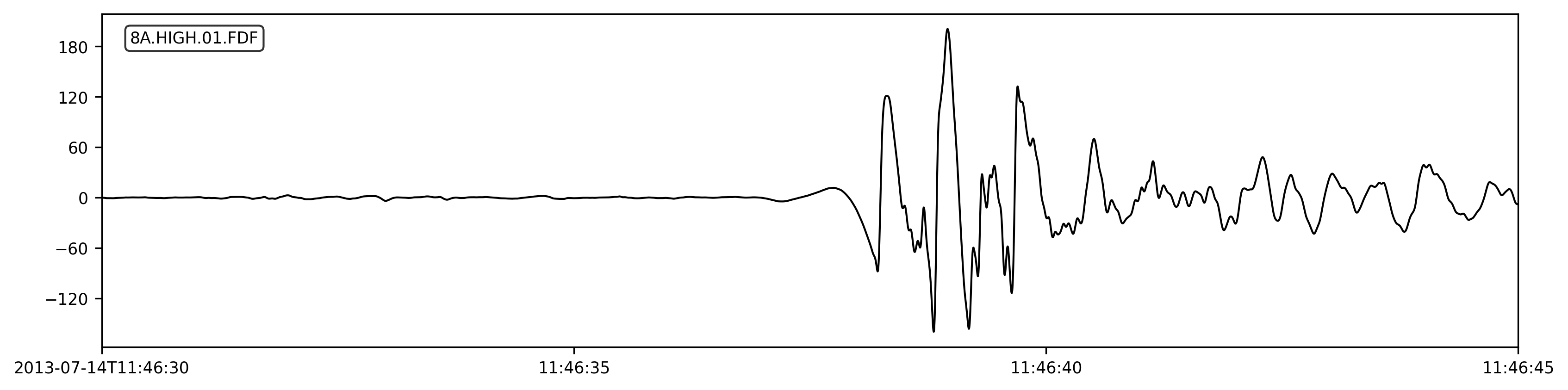
Coupled with the seismic sensors around Tungurahua are infrasound sensors that record atmospheric pressure. During the 2014 eruption, these sensors recorded this signal (band-pass filtered between 1 and 20 Hz) at the “HIGH” stations about 2 km from the conduit outlet.
Our goal was to couple the atmosphere to our volcano model to create a second source—in addition to seismic data—to validate our model against. I approached the atmospheric modeling problem using three methods, aiming to get comparable results from each method or at least understand any differences in output.
3.1 Quail atmospheric model (in progress)
Our first concept was to apply the axisymmetric atmospheric model that former PhD student Fred Lam had already implemented in Quail. Two challenges with the Quail implementation are: (1) it is very hard to validate, and (2) adding the atmosphere affects the 1D volcano model in the conduit, which is certainly incorrect. As of this writing, I am still working to better understand what is happening here.
3.2 Simple monopole source model
In order to sanity check the output of the Quail atmosphere model, we decided to create a very simple atmosphere model where we assume the source term to be a single monopole at the outlet of the volcano from which pressure could be modeled with the relation:
\[p(r,t) = \frac{\rho \dot{Q}(t-r/c)}{4 \pi} \\\]where $Q(t) = \dot{s} \pi R^2$ is the volumetric flow in units $[\frac{m^3}{s}]$. The derivation for this relation can be found here. The code for this simple model is in my weekly notes from April.
Monopole source model applied to the simple slip eruption in section 1.
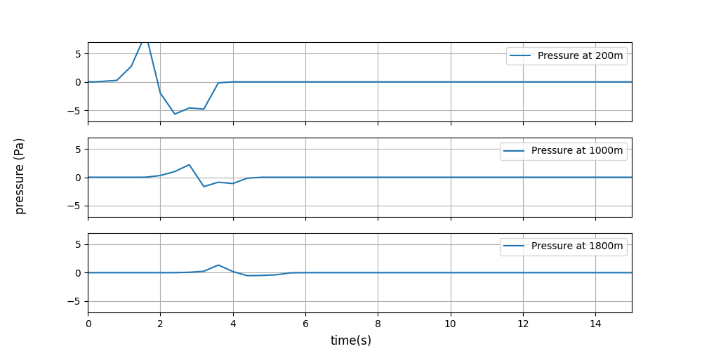 Pressure measured at various distances from the outlet for the above simulation.
3.3 Lighthill Stress Tensor (in progress)
One challenge with the quail atmosphere model is that the error term is fairly diffusive. One way of getting around the diffusive error is to use the Lighthill Analogy where Lighthill rearranged the Navier-Stokes equation into an inhomogenous wave equation where the source term only exists in regions of turbulent flow.
\[\begin{align} \frac{1}{c_0^2}\frac{\partial^2p}{\partial t^2} - \nabla^2 p = \nabla \cdot (\nabla \cdot T) \\ \end{align}\]The free-space Green’s theorem satisfies the case
\[\begin{align} \frac{1}{c_0^2}\frac{\partial^2 G}{\partial t^2} - \nabla^2 G = 0 \end{align}\]where the free-space Green’s theorem for three dimensions is given by
\[\begin{align} G(x, t; y, \tau) = \frac{\delta( t - \tau - \frac{|x-y|}{c0})}{4 \pi |x - y|} \end{align}\]Volume Integral approach
The simplest approach for calculating pressure with the Lighthill analogy is to integrate over the entire volume of turbulent flow and use that volume integral to predict the acoustic pressure at some distant location $x$.
\[\begin{align} p'(x,t) &= \int \int_V G(x, t; y, \tau) \frac{\partial^2 T_{ij}}{\partial y_i \partial y_j}(y, \tau)dy d\tau \\ p'(x,t) &=\frac{1}{4 \pi} \int_V \frac{1}{|x-y|} \frac{\partial^2 T_{ij}}{\partial y_i \partial y_j}(y, t-\frac{|x-y|}{c_0})dy^3 \end{align}\]Volume Integral verification:
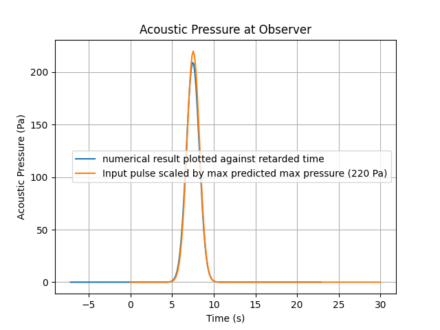
To verify that my code for solving the volume integral was indeed behaving as intended, I created a simple test with spatially constant, temporal gaussian substituting the double divergence of the lighthill stress tensor. In this case, because the source term is uniform across the volume $R < 100$ and $Y>0$ and $Y< 100$, we can write the equation for max pressure:
\[p_{max} = \frac{1}{4 \pi} \int_V \frac{1}{|x_{obs} - y|} dy\]That can roughly be approximated as
\[\begin{align} p_{max} =& \frac{1}{4 \pi} \frac{V}{r_{avg}} \\ p_{max} =& \frac{1}{4 \pi} \frac{\pi * 100^2 * 200}{2300} \\ p_{max} =& 220 [Pa] \end{align}\]And sure enough! When I plot the numerical output from the volume integral at retarded time against the input pulse scaled by $220$, I get matching gaussian curves!
The next step is to apply the volume integral approach to the double divergence of the lighthill stress tensor. I do that in my notes from the week of 2025.05.19. However, because I don’t trust my input, I also don’t trust my output.
Surface Integral approach:
It is also possible to translate the volume integral as a surface integral.
\[\begin{align} p'(x,t) = \frac{1}{4\pi} \int_v \frac{1}{|x - y|} \frac{\partial}{\partial y_i} \frac{\partial T_{ij}}{\partial y_j} (y, t - \frac{|x-y|}{c_0}) dy^3 \end{align}\]Applying the divergence theorem, we can rewrite this volume integral as a surface integral.
\[\begin{align} p'(x,t) = \frac{1}{4\pi} \int_S \frac{1}{|x - y|} \frac{\partial T_{ij}}{\partial y_j} (y, t - \frac{|x-y|}{c_0}) \cdot \hat{n} dy^2 \end{align}\]Let’s integrate over the sphere with a radius $a=100m$. Let’s review a couple aspects of spherical coordinates.
\[\begin{align} dS =& a^2 \sin \phi d \phi d \theta \\ x =& a \sin \phi \cos \theta \\ y =& a \sin \phi \sin \theta \\ z =& a \cos \phi \end{align}\]So we should be able to rewrite the surface integral as follows:
\[p'(x, t) = \frac{1}{4 \pi} \int_0^{\pi/3} \int_0^{2\pi} \frac{1}{|x - y|} \frac{\partial T_{ij}}{\partial y_j} n_j a^2 \sin \phi d \phi d \theta\]4.0 Conclusion
I have enjoyed working on these various projects related to Mario’s work on accurately simulating the Tungurahua eruption. I will continue to update this page as additional developments occur.
Leave a Comment
Your email address will not be published. Required fields are marked *