2025.08.22 GNC Interview Prep

1. Orbital Mechanics

1.1. Write orbital simulator (Kepler's problem)

import numpy as np
from scipy.integrate import solve_ivp
import matplotlib.pyplot as plt

# Constants
mu = 3.986004418e14           # Earth's gravitational parameter [m^3/s^2]
Re = 6378137.0                # Earth's equatorial radius [m]
J2 = 1.08263e-3               # J2 coefficient

def j2_accel(r_vec):
    x, y, z = r_vec
    r = np.linalg.norm(r_vec)
    zx = z / r
    factor = 1.5 * J2 * mu * Re**2 / r**5

    ax = factor * x * (5 * zx**2 - 1)
    ay = factor * y * (5 * zx**2 - 1)
    az = factor * z * (5 * zx**2 - 3)
    return np.array([ax, ay, az])

def two_body_j2(t, state):
    r = state[0:3]
    v = state[3:6]
    r_norm = np.linalg.norm(r)

    # Gravity + J2
    a_gravity = -mu * r / r_norm**3
    a_j2 = j2_accel(r)

    a_total = a_gravity #+ a_j2
    return np.concatenate((v, a_total))

# Initial state (example: circular orbit at 500 km altitude)
altitude = 500e3
r0 = Re + altitude
v0 = np.sqrt(mu / r0)

# Place satellite at x=r0, moving in y
state0 = np.array([r0, 0, 0, 0, v0, 0])

# Time span for simulation (1 orbit ~ 5400 s)
T_orbit = 2 * np.pi * np.sqrt(r0**3 / mu)
t_span = (0, 10 * T_orbit)  # simulate 10 orbits
t_eval = np.linspace(*t_span, 10000)

# Solve ODE
sol = solve_ivp(two_body_j2, t_span, state0, t_eval=t_eval, rtol=1e-8)

# Extract results
x, y, z, vx, vy, vz = sol.y[0], sol.y[1], sol.y[2], sol.y[3], sol.y[4], sol.y[5]

# Plot
fig = plt.figure(figsize=(6,6))
ax = fig.add_subplot(111, projection='3d')
ax.plot(x/1000, y/1000, z/1000)
ax.set_title("Orbital Trajectory with J2 Perturbation")
ax.set_xlabel("X [km]")
ax.set_ylabel("Y [km]")
ax.set_zlabel("Z [km]")
plt.tight_layout()
plt.show()

1.2 Simulate gps measurement with gaussian noise

# Set GPS noise level (e.g. 100 m standard deviation)
gps_noise_std = 100000.0  # meters

# Stack true positions
true_state = np.vstack((x, y, z, vx, vy, vz)).T  # shape: (n_samples, 3)

# Simulate GPS measurements with Gaussian noise
noisy_state = true_state + np.random.normal(0, gps_noise_std, size=true_state.shape)

# Plot true vs. noisy GPS for visualization
import matplotlib.pyplot as plt

plt.figure(figsize=(8,6))
plt.plot(true_state[:,0]/1000, true_state[:,1]/1000, label="True Orbit")
plt.plot(noisy_state[:,0]/1000, noisy_state[:,1]/1000, '.', markersize=1, label="Noisy GPS")
plt.xlabel("X [km]")
plt.ylabel("Y [km]")
plt.legend()
plt.title("Simulated GPS Measurements (2D View)")
plt.grid()
plt.axis("equal")
plt.show()

1.3 Write a Kalman filter

• $F$ - transition matrix
• $Q$ - Process covariance (unmodeled acceleration, imperfect numerical integration)
• $R$ - Measurment covariance
• $P$ - State covariance
• $S$ - inovation corvariance

Prediction step:

$$ \begin{align} x &= f(x, dt) \\ F &= F(x, dt) \\ P &= F P F^T + Q \end{align} $$

We want to propagate the current state estimate and the current covariance estimate.

Update step:

$$ \begin{align} y = z - x \\ S = P + R \\ K = P S^{-1} \\ x = x + Ky \\ \end{align} $$

The biggest open question to me in this sequence is the derivation of how we solve for kalaman gain as $ P S^{-1}$. I am not reproducing here, but that can be dervivied by minimizing the error covariance.

import numpy as np

def f(x, dt):
    """
    State transition function for constant velocity model.
    x: current state vector [x, y, z, vx, vy, vz]
    dt: time step
    """
    derivative = two_body_j2(0, x)  # acceleration at current state

    return x + derivative * dt

def F_jacobian(state, dt):

    return np.eye(6) + np.diag(two_body_j2(0, state)) * dt

def extended_kalman_filter_pos_vel(f, F_jacobian, zs, dt, R, Q):
    n = zs.shape[0]
    x_est = np.zeros((n, 6))  # state estimates: [x, y, z, vx, vy, vz]
    y_est = np.zeros(n)        # innovation norms
    P = np.eye(6) * 1e3       # initial state covariance

    # Initial state guess from first measurement
    x = zs[0]

    for k in range(n):
        # --- Prediction ---
        x = f(x, dt)
        F = F_jacobian(x, dt)
        P = F @ P @ F.T + Q

        # --- Update ---
        z = zs[k]
        y = z - x                   # innovation
        S = P + R             # innovation covariance
        K = P @ np.linalg.inv(S)  # Kalman gain
        x = x + K @ y
        P = (np.eye(6) - K) @ P

        x_est[k] = x
        y_est[k] = np.linalg.norm(y)

    return x_est, y_est

x_est, errors = extended_kalman_filter_pos_vel(f, F_jacobian, noisy_state, dt=5.677545, R=np.eye(6) * gps_noise_std**2, Q=np.eye(6) * 1e-3)

plt.figure(figsize=(8,6))
#plt.plot(true_state[:,0]/1000, true_state[:,1]/1000, label="True Orbit")
#plt.plot(noisy_state[:,0]/1000, noisy_state[:,1]/1000, '.', markersize=1, label="Noisy GPS")
plt.plot(x_est[:,0]/1000, x_est[:,1]/1000, label="EKF Estimate", color='red')
plt.xlabel("X [km]")
plt.ylabel("Y [km]")
plt.legend()
plt.title("Simulated GPS Measurements (2D View)")
plt.grid()
plt.axis("equal")
plt.show()

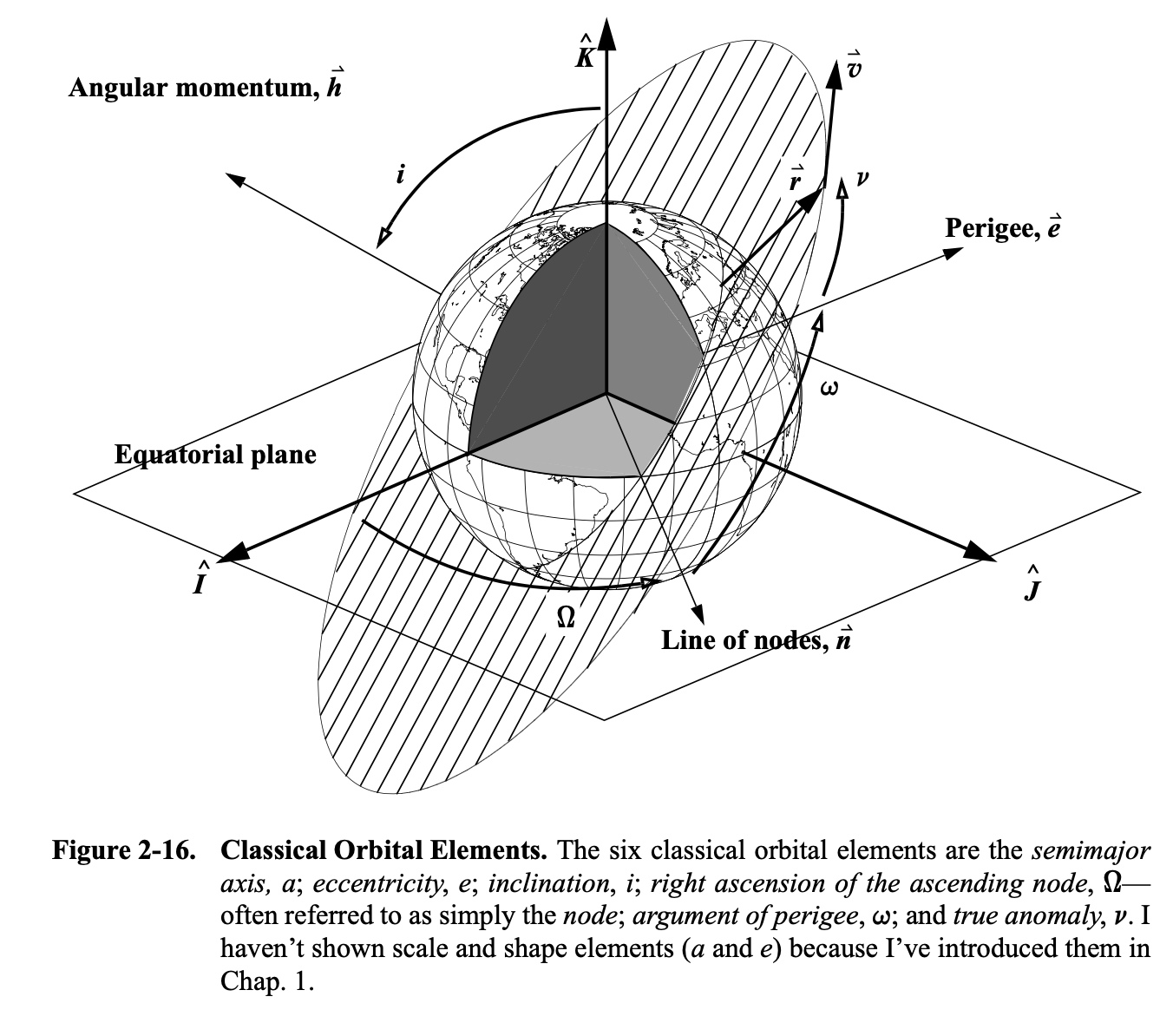
2. Vocabulary

2.1 Orbital Dynamics vocabulary

Term	Definition
Anomaly (True Anomaly, $\nu$)	The angle between the direction of periapsis and the current position of the satellite, measured in the orbital plane. Describes where the spacecraft is in its orbit.
Right Ascension of the Ascending Node (RAAN, $\Omega$)	The angle from the inertial X-axis to the ascending node (where the orbit crosses the equatorial plane from south to north). Measured in the equatorial plane.
Argument of Perigee ( $\omega$ )	The angle from the ascending node to the orbit’s closest point to Earth (perigee), measured in the orbital plane.
Inclination ( $i$ )	The tilt of the orbital plane with respect to Earth’s equatorial plane.
Eccentricity ( $e$ )	Describes the shape of the orbit: 0 is circular, between 0 and 1 is elliptical.
Semi-Major Axis ( $a$ )	Half the longest diameter of the orbital ellipse. Defines the orbit size.
Mean Anomaly ( $M$ )	A mathematical angle that increases linearly with time; used to compute position along the orbit.
Eccentric Anomaly ( $E$ )	An auxiliary angle used to relate mean and true anomaly via Kepler’s equation.
Perigee/Apogee	Closest and farthest points in the orbit from the central body.
Nodal Precession	Slow rotation of the orbit plane due to perturbations (e.g., Earth’s oblateness). Affects RAAN.
J2 Perturbation	A gravitational effect due to Earth’s equatorial bulge, causing orbital plane drift.

2.2 Reference frames

Term	Definition
Body Frame	Coordinate frame fixed to the spacecraft.
Inertial Frame (ECI)	Non-rotating frame relative to the stars; used for orbit propagation.
Orbital Frame (LVLH)	Local frame aligned with velocity and nadir direction.
ECEF (Earth-Centered, Earth-Fixed)	Frame fixed to Earth's surface; rotates with Earth.
RBC (Radial, Along-track, Cross-track)	Frame commonly used for relative motion in orbit.

2.3 Graphic with relative quantities labeled

Note, we need 6 state variables to fully describe an orbit. Those can take the form of:

• classical orbital elements
• osculating elements
• position/velocity (two body-elements)
• Keplarian elements

2.4 Perterbations

Perturbation	Source	Affects Which Orbital Elements?	Timescale	Typical Effect
J2 (Earth oblateness)	Earth's equatorial bulge	RAAN (Ω), Argument of Perigee (ω), Mean Anomaly (M)	Long-term secular	Nodal precession, perigee rotation
Atmospheric drag	Upper atmosphere	Semi-major axis (a), eccentricity (e)	Short-term & secular	Orbital decay, circularization
Solar radiation pressure	Photons from the Sun	Eccentricity (e), inclination (i), area-sensitive	Long-term periodic/secular	Small thrust, orientation-dependent
Third-body gravity	Sun, Moon (or other planets)	All elements (especially e, i, ω)	Long-term periodic	Precession, resonance effects
Relativistic effects	General relativity	Argument of Perigee (ω)	Very long-term	Tiny perigee advance
Earth tides	Deformation of Earth by Moon & Sun	Argument of Perigee (ω), semi-major axis (a)	Long-term	Very small
Albedo / IR radiation	Reflected sunlight / Earth IR	Similar to SRP	Long-term	Minor drag-like effect
Solar cycle	Sun’s 11-year cycle → atmospheric density changes	Drag (a, e)	Years	Modulates drag impact
Magnetic field effects	For charged spacecraft	Attitude/orbit (if affected)	Variable	Rare but possible

Basic mathmatical relations

Semi major axis

$$ a = (\frac{2}{r} - \frac{v^2}{\mu})^{-1} = \frac{r_a + r_p}{2} $$

Mean motion

$$ \begin{align} n = \sqrt{\frac{\mu}{a^3}} \\ \end{align} $$

where $\mu$ is the gravitation parameter.

Eccentricity

$$ e = \frac{\vec{v} \times \vec{h}}{\mu} - \frac{\vec{r}}{r} $$

The eccentricity vector always points at the periapsis.

Inclination

$$ \cos{i} = \frac{\hat{k} \cdot {\vec{h}}}{|\hat{k}||\vec{h}|} $$

Where k is just the unit vector in the z direction.

right ascension of ascending node (RAAN)

ascending node -- where Spacecraft crosses equitorial plane from south to north. The vector of the ascending node can be found with:

$$ \vec{n} = \hat{k} \times \vec{h} $$

We can see equitorial orbits have no ascending node.

Argument of perigee

Angle measured from the ascending node to the closest point of the orbit.

$$ \cos{\omega} = \frac{\vec{n} \cdot \vec{e}}{|\vec{n}||\vec{e}|}$$

This is undefined for circular and equitorial orbits.

True anomaly

$$\cos{\nu} = \frac{\vec{e} \cdot \vec{r}}{|\vec{e}||\vec{r}|}$$

satellite location relative to the perapsis.

Velocity

Note, that velocity is just a function of semi-major axis, gravitational parameter, and current location.

$$ v = \sqrt{\frac{2 \mu}{r} - \frac{\mu}{a}}$$

Energy

(Below is for a circular orbit) $$ \begin{align} \epsilon &= \frac{v^2}{r} - \mu r \\ \epsilon &= - \frac{\mu}{2r} \end{align} $$

Time

• epoch - specific moment

• Sidereal day - 23h 56m 4.1s

• Mean solar time(UT1) - based on ficitious mean Sun, defined as a function of Sidereal time.

• Atomic time (TAI) = spaced on the specific quantum transitions of electrons in a cesium-133 atom. The transition emits photons at a known frequency that we can count.

• Coordinated universal time (UTC) - derived from ensemble of atomic clocks. UTC originated in 1962. 27 leap seconds have been added since 1972, keeps UTC reasonably close to UT1 (mean solar time).

• GPS time - the GPS epoch is Jan 6, 1980 0hr UTC time. GPS time is not adjusted by leap seconds.

Maneuvering

Gauss Planetary Equations The Gauss planetary equations describe the time rate of change of the classical orbital elements under a perturbing acceleration in the orbital frame, with components radial ($a_r$), tangential ($a_t$), and normal ($a_n$). The orbital elements are semi-major axis ($a$), eccentricity ($e$), inclination ($i$), right ascension of the ascending node ($\Omega$), argument of perigee ($\omega$), and mean anomaly ($M$). The equations assume a central gravitational field with parameter $\mu$, semi-latus rectum $p = a (1 - e^2)$, and radial distance $r = \frac{p}{1 + e \cos \theta}$, where $\theta$ is the true anomaly.

Orbital Element Derivative with Respect to Time ($\frac{d}{dt}$)

Semi-major axis ($a$) $\frac{2a^2}{\sqrt{\mu p}} \left[ e \sin \theta \cdot a_r + \frac{p}{r} \cdot a_t \right]$

Eccentricity ($e$) $\frac{1}{\sqrt{\mu p}} \left[ p \sin \theta \cdot a_r + \left( (p + r) \cos \theta + r e \right) \cdot a_t \right]$

Inclination ($i$) $\frac{r \cos (\theta + \omega)}{\sqrt{\mu p}} \cdot a_n$

Right Ascension of the Ascending Node ($\Omega$) $\frac{r \sin (\theta + \omega)}{\sqrt{\mu p} \sin i} \cdot a_n$

Argument of Perigee ($\omega$) $\frac{1}{\sqrt{\mu p} e} \left[ -p \cos \theta \cdot a_r + (p + r) \sin \theta \cdot a_t \right] - \frac{r \sin (\theta + \omega) \cos i}{\sqrt{\mu p} \sin i} \cdot a_n$

Mean Anomaly ($M$) $n - \frac{1 - e^2}{\sqrt{\mu p} e} \left[ \left( p \cos \theta - 2 e r \right) \cdot a_r - (p + r) \sin \theta \cdot a_t \right]$, where $n = \sqrt{\frac{\mu}{a^3}}$

Notes

Parameters: $a$: Semi-major axis $e$: Eccentricity $i$: Inclination $\Omega$: Right ascension of the ascending node $\omega$: Argument of perigee $\theta$: True anomaly $\mu$: Gravitational parameter (e.g., ~398,600 km³/s² for Earth) $p = a (1 - e^2)$: Semi-latus rectum $r = \frac{p}{1 + e \cos \theta}$: Radial distance $n = \sqrt{\frac{\mu}{a^3}}$: Mean motion

Acceleration Components: $a_r$: Radial acceleration (toward the central body) $a_t$: Tangential acceleration (along the velocity vector, in-track) $a_n$: Normal acceleration (perpendicular to the orbital plane, out-of-plane)

Usage: These

Coplanar maneuvers

• Change semimajor axis
• change ecentricity
• Coplanar burns are either tangential or non-tangential
• For max efficiency, burns either occur at appoapsis or perapsis.

Hohmann Transfer

• Two burns 1/2 orbit apart. First tangential burn places the satellite into an eliptical pattern, the second burn slightly circulerizes.

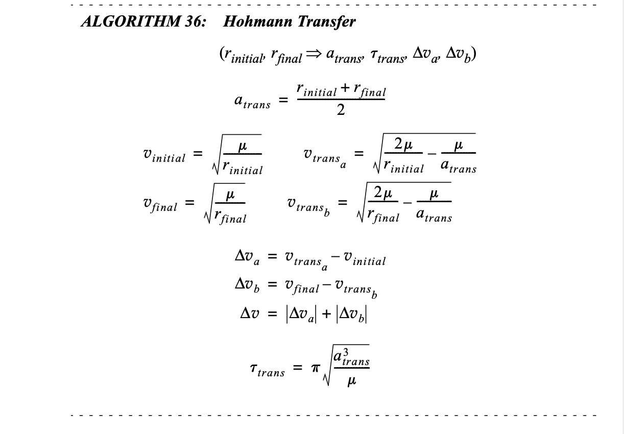
Example question

A satellite is initially in a circular low Earth orbit (LEO) at an altitude of 700 km. You want to transfer it to a higher circular orbit at an altitude of 35,786 km (geostationary orbit).

1. Compute the Δv for the first burn (from LEO to the transfer ellipse).
2. Compute the Δv for the second burn (to circularize at GEO).
3. Compute the total Δv required for the Hohmann transfer.

r_i = 7000e3  # Initial radius in meters
r_f = 35786e3 # Final radius in meters
mu = 3.986004418e14  # Gravitational parameter for Earth in m^3/s^2
R = 6371e3  # Radius of Earth in meters

a_trans = (r_i + r_f) / 2  # Semi-major axis of transfer orbit

v_i = np.sqrt(mu/r_i)
v_f = np.sqrt(mu/r_f)

v_trans_a = np.sqrt(2 *mu / r_i - mu/a_trans)
v_trans_b = np.sqrt(2 *mu / r_f - mu/a_trans)

dv_a = v_trans_a - v_i
dv_b = v_f - v_trans_b

total_dv = dv_a + dv_b

print(f"Total Delta-V for Hohmann Transfer: {total_dv/1000:.2f} km/s")
print(f"First burner Delta-V: {dv_a/1000:.2f} km/s")
print(f"Second burner Delta-V: {dv_b/1000:.2f} km/s")

print(f"Initial velocity: {v_i/1000:.2f} km/s")
print(f"Final velocity: {v_f/1000:.2f} km/s")

print(f"Total circumference of Earth: {2 * np.pi * R/1000:.2f} km")

print(" ")
print(f"Initial energy: {(1/2 * v_i**2  - mu/(r_i))/1e6:.2f} MJ/kg")
print(f"Final energy: {(1/2 * v_f**2 - mu/(r_f))/1e6:.2f} MJ/kg")


energy_dv1 = (1/2 * v_trans_a**2 - 1/2 * v_i**2)
energy_dv2 = (1/2 * v_f**2 - 1/2 * v_trans_b**2)

print(f"Total energy from delta_vs: {(energy_dv1 + energy_dv2)/1e6:.2f} MJ/kg")

Total Delta-V for Hohmann Transfer: 3.64 km/s
First burner Delta-V: 2.21 km/s
Second burner Delta-V: 1.43 km/s
Initial velocity: 7.55 km/s
Final velocity: 3.34 km/s
Total circumference of Earth: 40030.17 km
 
Initial energy: -28.47 MJ/kg
Final energy: -5.57 MJ/kg
Total energy from delta_vs: 22.90 MJ/kg

Inclination changes

Because Astranis launches their satellites our of Cap Canavaral at ~28 degrees or so, we also need to execute an out of plan burn.

$$ \begin{align} \Delta v_1 &= 2 v_2 \sin{\frac{\Delta i}{2}} \\ \Delta v_1 &= 2 * (3.34 km/s) * \sin{\frac{28.5 deg}{2}} \\ \Delta v_1 &= 2 * 3.34 * 0.25 [km/s] \\ \Delta v &= 1.67 [km/s] \end{align} $$

Non-coplanar transfers

• Out of plan burn changes $i$ and $\Omega$ (RAAN)
• Applying an out-of-plane burn at nodal crossing will only change inclination. An other out of plane burn will change both inclination and RAAN.
• Launch sites limit inclination or launch. The iniclination of a satellite must be greater than the lattitude of the launch site, or an out of plane burn in orbit must be used.
• Changing the inclination of an eliptical orbit also ends up changing the location of the ascending node as well.

Impulsive vs continuous thrust

Basic idea of continous thrust solutions:

1. Write out state equations.
2. Define cost functions.
3. Solve control law.

Optimal control theory

• write out a hamiltonian with a cost function (like magnitude of velocity) and $\lambda$ term attached to the dynamics. In doing this, you can see how much energy is required to make a small change in outcome.

Launch windows

• Selected to get correct RAAN

Sun Synchronous

• 98 degrees, slightly retrograde orbit.
• Needs to be retrograde to produce eastward precession.

Misc technical question

1. Describe what a GNC system is and how the components interact?
   Guidance -> determine desired trajectory Navigation -> estimates satellites current trajectory (GPS, IMU, startrack) Control -> generates control response (thrusters + IMUS + magnetorqers)

2. Relevant algorithms? EXF - extended kalaman filter (extended refers to dealing with non-linear systems) PID - proportional integral-derivative controller, a controller that picks a value based on constant multiples of integral, variable, and derivative of variable. Tune parameters manually. LQR - Solves for K ( u = -Kx) by minimizing quadratic cost function. Optimal, based on minimizing cost function

3. How would you estimate spacecraft attitude using star tracker and gyro data? Kalman filter State vector -> quaternion q + gyro bias Prediction step -> propagate attitude Update step -> use star tracker measurement to update estimate

4. What causes attitude instability? poorly tuned gains Actuator saturation or failure

5. Walk me through how you would design a control loop for a satellite attitude control system. What components are essential?

   • First you want a target, planned attitude
   • Then you would need a way of measuring attitude (IMU)
   • Next a MEKF in order smooth out the noisy measurments
   • Then you would want to close the loop with some kind of PID control system.
   • You could use LQR to find an optimal control strategy.

6. What are the tradeoffs between using reaction wheels, control moment gyros, and thrusters for attitude control?

   • reaction wheels are the best but can become saturated.
   • thrusters good to unsaturate reaction wheels.

7. How does a Kalman Filter work, and where might it be used on a spacecraft?

   • Basic idea is to have a prior with some covariance matrix. And then except new measurments also with covariance. And then weigh the confidence in the predicted state vs the confidence in the newly measured state to inform the final solution.

8. Can you explain how a quaternion represents orientation and why it's preferred over Euler angles in space applications?

   • quaternions are vectors of vector of length 4, describes rotation from 1 frame to another.
   • Common use is to convert a vector from one frame to a different frame. That can be done by simple quaternion multiplication.
   • preffered in part because avoids gyro lock.
   • also more efficient computation that euler angels

9. What are the stability conditions for a linear time-invariant (LTI) system? How would you test stability in a nonlinear system?

   • negative eigenvalues.
   • Non-linear system you would want to linearize about a specific point.

10. How would you model the effects of gravity gradient torque on a spacecraft in GEO?

    • Yeah create a torque. Need to review book for mathmatics specifics.

11. Describe how you would use a star tracker and a gyro together for attitude estimation.

    • startracker slow update, but accurate.
    • gryo fast update but can drift over time
    • use startrack to periodically reset gyro drift, this could be done with some form of KF or EKF.

12. What is the role of a B-dot controller in detumbling?

    • magnetetic control law used to passively stabalize sat

13. How would you design an Extended Kalman Filter to estimate both position and velocity using noisy GPS data?

    • See above.

14. What's the difference between the process noise and measurement noise covariance matrices in a Kalman filter?

    • process noise -- numerical errors + factors we are not modeling (added to predictive state covariance)
    • measurment -- errors in recording sensor (added to to measurment covariance)

15. Have you used Monte Carlo simulations to validate your GNC algorithms? What were you testing for?

    • Monte Carlo sim "dart throwing" sim.
    • I don't think I've ever used it for a GNC alg, but I had used it to calculate Pi.

16. How would you simulate a spacecraft's orbit with J2 perturbation included?

    • If I was simulating the spacecraft with postion/velocity, I would just add an additional acceleration term. An example is above.

17. Write or describe the equations of motion for a spacecraft in Earth orbit including perturbative effects.

    • J2 effect (causes RAAN precession)
    • Atmospheric drag for satellites in lower orbit (causes drop in SMA, also slight circulerizing effect for sats in eliptical orbit)
    • Solar radiation pressure
    • third body perturbations ()
    • Earth tides + relativistic effects.

18. Let’s say your satellite is slowly spinning in GEO and your sensors are misbehaving — how would you begin debugging the issue?

    • check telemetry for sensor health
    • compare outputs of star tracker vs gryro
    • check acuators
    • Try to change attitude of satellite to a more stable orientation

19. If your Kalman filter starts diverging in flight, what might be the causes?

    • Incorrect covariance for measurment noise/process noise?
    • sensor failures
    • numerical error

20. How would you validate that your attitude estimation algorithm is working correctly on orbit with limited telemetry?

    • Downlink attitude estimates
    • Cross check different sensors with final output

21. Would you prefer to use a model-based or data-driven approach to build a new controller? Why?

    • Model based sounds better if it considers the actual physics.

Practice coding challenge: implement j2 orbit propagation

from  scipy.integrate import solve_ivp

mu = 398600.4418  # km^3/s^2
R = 6378.137      # km
J2 = 1.08263e-3

def gravity_accel(r_vec):
    """
    Computes the gravitational acceleration vector at position r_vec.
    
    Parameters:
        r_vec (np.ndarray): Position vector [x, y, z] in ECI frame (km)
        
    Returns:
        np.ndarray: Gravitational acceleration vector [ax, ay, az] in km/s^2
    """
    r_norm = np.linalg.norm(r_vec)

    a_gravity = -mu * r_vec / r_norm**3

    return a_gravity

def j2_accel(r_vec):
    """
    Computes the Jacobian of the J2 acceleration with respect to position.
    
    Parameters:
        r_vec (np.ndarray): Position vector [x, y, z] in ECI frame (km)
        
    Returns:
        np.ndarray: Jacobian matrix of J2 acceleration (3x3)
    """
    x, y, z = r_vec
    r_norm = np.linalg.norm(r_vec)

    const_mult = 3 * J2 * mu * R**2 / (2 * r_norm**5)

    a_j2 = np.zeros(3)
    a_j2[0] = const_mult * x * (1 - 5 * (z**2 / r_norm**2))
    a_j2[1] = const_mult * y * (1 - 5 * (z**2 / r_norm**2))
    a_j2[2] = const_mult * z * (3 - 5 * (z**2 / r_norm**2))

    return a_j2

def state_dot(t, state):
    r_vec = state[0:3]
    v_vec = state[3:6]

    state_dot = np.zeros(6)

    state_dot[0:3] = v_vec
    state_dot[3:6] = gravity_accel(r_vec) + j2_accel(r_vec)

    return state_dot

def propagate_orbit_j2(state0, t_final, dt):
    """
    Propagates the orbit of a satellite using RK4 integration with J2 perturbation.

    Parameters:
        state0 (np.ndarray): Initial state vector [x, y, z, vx, vy, vz] in ECI frame (km, km/s)
        t_final (float): Final time in seconds
        dt (float): Time step in seconds

    Returns:
        times (np.ndarray): Array of time stamps
        states (np.ndarray): Array of propagated states (N x 6)
    """

    t_eval = np.linspace(0, t_final, t_final//dt)

    sol = solve_ivp(state_dot, y0=state0, t_span=[0,t_final], t_eval=t_eval, method='RK45',)

    return sol.t, sol.y

state0 = np.array([7000, 0, 0, 0, 7.5, 1.0])  # ECI position [km] and velocity [km/s]
t_final = 3600  # 1 hour
dt = 10         # 10-second step

times, states = propagate_orbit_j2(state0, t_final, dt)

r_sol = states[0:3]
v_sol = states[3:6]

ax = plt.figure().add_subplot(projection='3d')

# Plot a sin curve using the x and y axes.
x = states[0, :] / 1e3
y = states[1, :] / 1e3
z = states[2, :] / 1e3

ax.plot(x, y, z)
ax.set_xlabel("x [km]")
ax.set_ylabel("y [km]")
ax.set_zlabel("z [km]")

Text(0.5, 0, 'z [km]')

Relevant quantities

Angular momentum (vector)

$$h = r \times v$$

h = np.cross(r_sol.T, v_sol.T)

print(h.shape)

(360, 3)

Eccentricity (vector)

$$ e = \frac{1}{\mu} [ (||v||^2 - \frac{\mu}{r}) - (r \cdot v)v]$$

v_norm = np.linalg.norm(v_sol, axis=0)
r_norm = np.linalg.norm(r_sol, axis=0)

e1 = ((v_norm**2 - mu/r_norm)* r_sol)
e2 = (np.sum(r_sol * v_sol, axis=0) * v_sol)
e = 1/mu * (e1 - e2)

e_norm = np.linalg.norm(e, axis = 0)

print(e.shape)

(3, 360)

Inclination (scalar)

$$ i = \cos^{-1}{\frac{h_z}{||h||}}

i = np.arccos(h[:,2]/np.linalg.norm(h, axis=1))

print(i.shape)

plt.plot(times, i)

(360,)

[<matplotlib.lines.Line2D at 0x11680b250>]

Node vector

Vector that points towards the ascending node. $$ \vec{n} = \hat{k} \times \vec{h} $$

k = np.zeros((360, 3))
k[:,2] = 1

n_vec = np.cross(k, h, axis = 1)

n = np.linalg.norm(n_vec, axis=1)

print(n_vec.shape)

(360, 3)

Right ascension of ascending node

$$ \Omega = \cos^{-1}{(\frac{n_x}{||n||})} $$

Omega = np.arccos(n_vec[:,0] / n)

Omega.shape

plt.plot(times, Omega)

[<matplotlib.lines.Line2D at 0x1167c7250>]

Argument of periapsis

$$ \omega = \cos^{-1}{(\frac{\vec{n} \cdot \vec{e}}{ne})}

omega = np.arccos(np.sum(n_vec * e.T, axis=1) / (n * e_norm))

omega.shape

plt.plot(times, omega)

[<matplotlib.lines.Line2D at 0x11692d810>]

True anomaly

$$ \nu = \cos^{-1} ( \frac{\vec{e} \cdot \vec{r}}{e r}) $$

nu = np.arccos(np.sum(e * r_sol, axis=0) / (e_norm * r_norm))

plt.plot(times, nu)

[<matplotlib.lines.Line2D at 0x1169b9bd0>]

semi-major axis

$$\epsilon = \frac{v^2}{2} - \frac{\mu}{r}$$

epsilon = v_norm**2 / 2 - mu / r_norm

a = - mu / 2 * epsilon


plt.plot(times, a)

[<matplotlib.lines.Line2D at 0x116a41090>]

Practice problem 2: Kalman Filter

true_state = states
true_position = true_state[0:3,:]
true_velocity = true_state[3:6, :]

def generate_measured_state(true_state, H, nu_k): 
    measured_state = H @ true_state + np.random.normal(0, nu_k, (H @ true_state).shape)

    return measured_state

def generate_transition_matrix(state, dt):
    r_norm = np.linalg.norm(state[0:3])
    x = state[0]
    y = state[1]
    z = state[2]

    pa_pr = 3/r_norm**5 * np.array([
        [x**2, x*y, x*z],
        [x*y, y**2, y*z],
        [x*z, y*z, z**2]
    ]) - 1/r_norm**3 * np.eye(3)

    A = np.block([
        [np.zeros((3,3)),  np.eye(3)],
        [ pa_pr, np.zeros((3,3))]
    ])

    F = A*dt + np.eye(6)

    return F

def kalman_filter(measured_states, omega_k, nu_k, H, dt, x0):
    # first prediction is just the measured state 
    x = x0

    # Process covariance, including uncertainty of both process model and numerical error.
    # Of size 6 because we propagate both position and velocity.
    Q = np.eye(6) * omega_k

    # Measurment covariance, diag of 3 because we only measure position
    R = np.eye(3) * nu_k

    # State covariance
    P = np.eye(6) * nu_k 

    xs = np.zeros((6, measured_states.shape[1]))

    for i, z in enumerate(measured_states.T):
        # Predict 
        F = generate_transition_matrix(x, dt)

        x = F @ x  # propagate 
        P = F @ P @ F.T + Q

        # Update 
        epsilon = z - H @ x
        S = H @ P @ H.T + R 
        K = P @ H.T @ np.linalg.inv(S)
        x = x + K @ epsilon
        P = (np.eye(6) - K @ H) @ P

        xs[:,i] = x

    return xs

# measurment noise std
nu_k = 100 # [m]

# process noise std
omega_k = 0.01 # [m]

# Measurement matrix, only measure position
H = np.zeros((3, 6))
H[0, 0] = 1
H[1, 1] = 1
H[2, 2] = 1

# dt is set to 10 seconds from our truth solution 
dt = 10

#seed with initial state 
state0 = np.array([7000, 0, 0, 0, 7.5, 1.0])  # ECI position [km] and velocity [km/s]

measured_states = generate_measured_state(true_state, H, nu_k)

#generate_state_transition_matrix(measured_state[:,0]).shape

filter_states = kalman_filter(measured_states, omega_k, nu_k, H, dt, state0)

plt.plot(times, true_state[0,:], label="True")
plt.plot(times, measured_states[0,:], label="Measured")
plt.plot(times, filter_states[0, :], label="Filtered")
plt.legend()

<matplotlib.legend.Legend at 0x117479e50>